8E · Vascular Flow (Q)
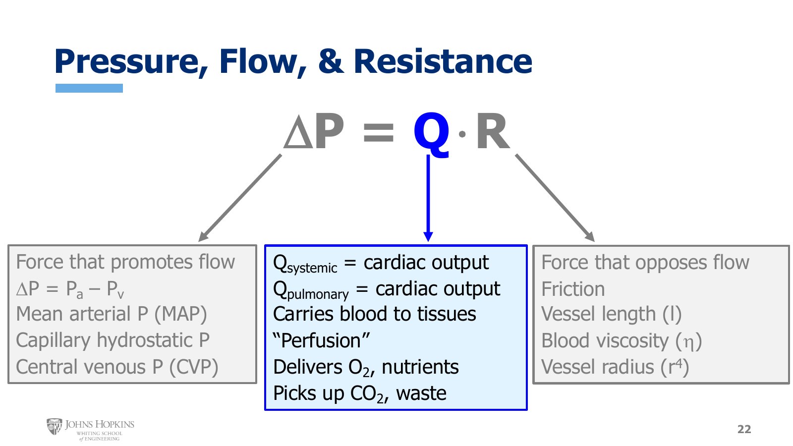
Slide 22. The overview again, now with Q highlighted: cardiac output, perfusion, and what flow delivers and picks up.
The big picture first. Flow is a critical factor in determining blood pressure. Flow for the entire systemic circulation coming out of the left ventricle is simply cardiac output, and flow for the entire pulmonary circulation coming out of the right ventricle is also cardiac output. Because right ventricular output determines and feeds into left ventricular output, the flow leaving each ventricle per minute is coupled, and both are called cardiac output.
This volumetric flow out of the ventricles and into the arteries is ultimately what carries blood to the tissues, and blood flow into the tissues of the body is also called perfusion. Tissue perfusion performs two critical jobs: deliver oxygen and nutrients to the tissues of the body, and pick up carbon dioxide and metabolic waste products from those tissues. Keep those big-picture purposes of flow in mind, even as we wade into the details that characterize and determine flow.
Flow in the ohmic framework
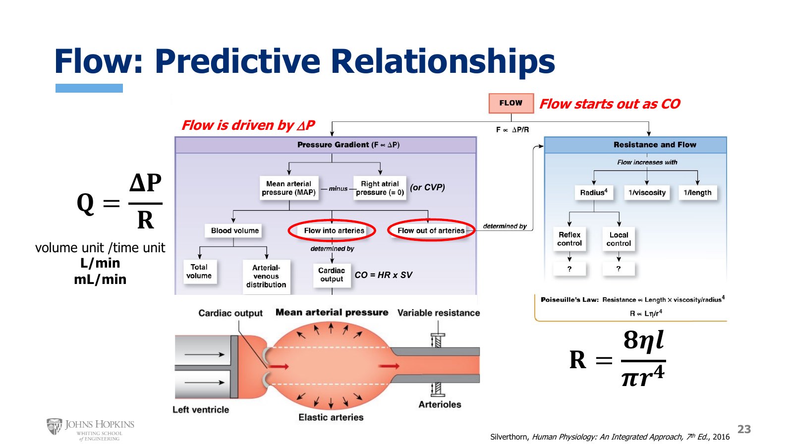
Slide 23. Flow is driven by ΔP and starts out as cardiac output. The flow chart traces mean arterial pressure back to blood volume, flow into the arteries, and flow out of the arteries, and resistance back to radius, viscosity, and length.
So far this module has considered flow through its traditional ohmic relationship with pressure and resistance.
Flow here is a volumetric flow rate, some measure of blood volume moving per unit time. In the body that is typically liters of blood per minute or milliliters of blood per minute.
Systemic flow starts out as cardiac output and is driven through the arteries, capillaries, and veins by a pressure gradient, always moving from a place of higher pressure to a place of lower pressure. Across the systemic circulation, that gradient is mean arterial pressure minus right atrial pressure, or central venous pressure. Since right atrial pressure and CVP are so low, nearly always close to zero, we really just need to look at mean arterial pressure to see the factors that influence the pressure gradient, and so influence the force that drives flow.
Mean arterial pressure is primarily influenced by three things:
Blood volume. Lecture 8D showed that blood volume distribution differs between arteries and veins, and that blood volume inside the vessel, along with that vessel’s inherent compliance, helps determine pressure inside it.
Flow into the arteries. Flow rates determine how much new blood enters a vessel each minute, and flow into the arterial side is pretty much determined by the flow leaving the ventricle, cardiac output. Think back to the heart module: every factor that influences heart rate or stroke volume impacts cardiac output, and so influences arterial inflow.
Flow out of the arteries. If cardiac output is the primary determinant of flow into the arteries, resistance is the primary determinant of flow leaving them. How hard is it for blood to flow out? Higher resistance means lower flow rates leaving the arteries. Lower resistance means higher flow rates leaving.
This lecture isn’t about resistance, but it is a chance to refresh the major physiological determinants of resistance from the rearranged Hagen-Poiseuille equation: vessel radius, particularly arteriolar radius (the screws controlling arteriolar dimensions in the figure), blood viscosity, and vessel length. Lecture 8F covers the control of vessel radius, and the relevance of viscosity and length, in much more detail.
Flow, velocity, and cross-sectional area
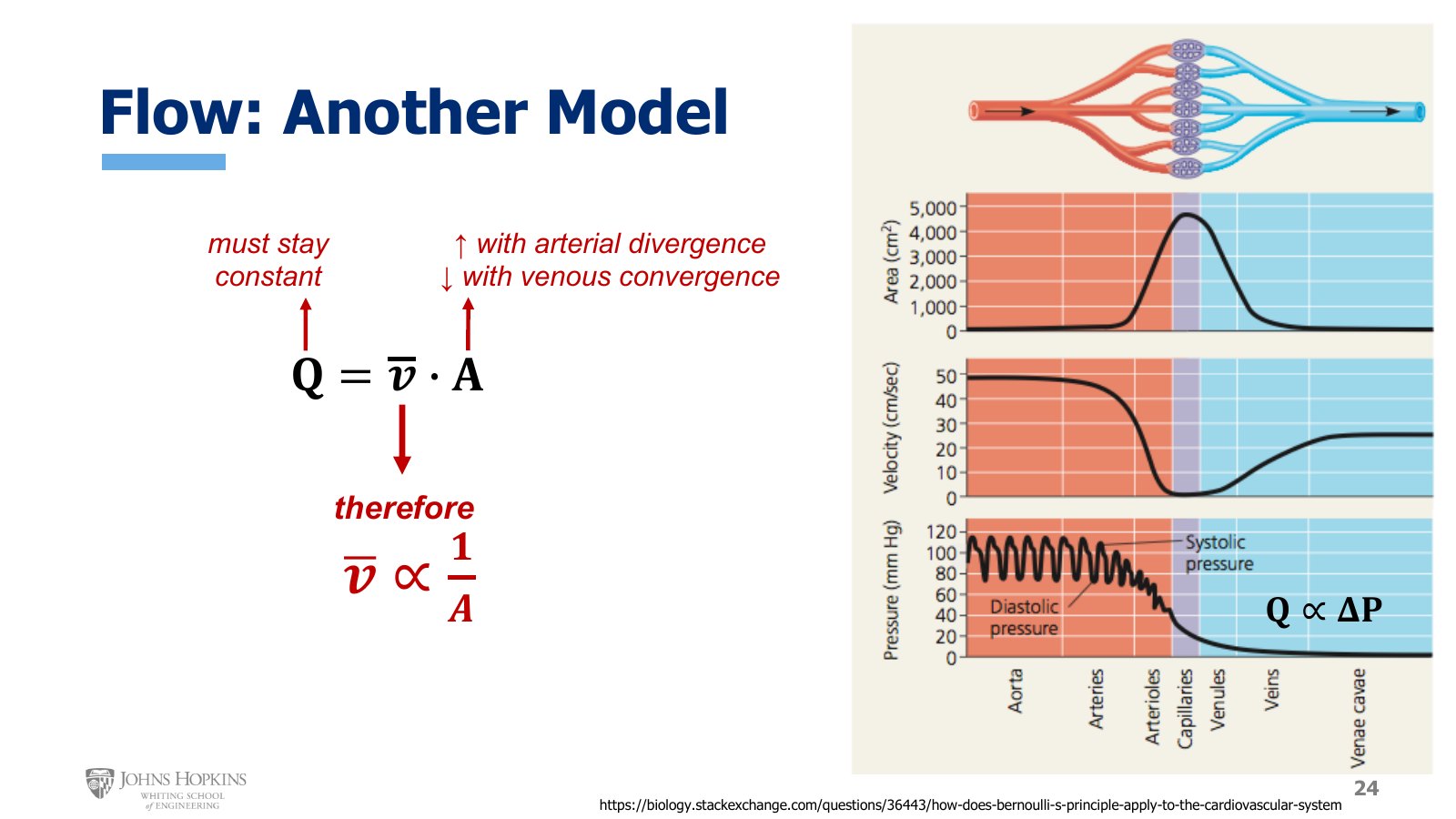
Slide 24. Aggregate cross-sectional area, mean velocity, and pressure from aorta to venae cavae. Area and velocity mirror each other.
Now step away from the ohmic framework and consider flow’s relationship with other vascular factors. This classic set of figures shows how aggregate cross-sectional area, blood velocity, and pressure change through the systemic circulation from aorta to vena cava.
The bottom figure appeared earlier in the module. It shows pulsatility dampening as blood travels farther from the left ventricle, and pressure starting high in the aorta and falling through the rest of the circulation. It reminds us of the systemic pressure gradient that drives flow from mean arterial pressure to central venous pressure.
The other two figures, velocity and cross-sectional area, have unique profiles: they mirror each other. Aggregate cross-sectional area is lowest in the large vessels and highest in the capillaries. Blood velocity is highest in the large vessels and lowest in the capillaries.
Aggregate cross-sectional area increases in the smaller vessels because there are just so many vessels at those levels. But why does blood velocity start out high, slow down, and then speed up again, especially when pressure keeps decreasing? Because of this relationship, flow equals mean blood velocity times aggregate cross-sectional area:
Q must stay constant through the entire circulation, because flow is conserved. The volumetric flow rate through a single aorta must equal the flow rate through the 10 billion downstream capillaries.
A changes depending on where we are, increasing through the arterial side with divergence and decreasing through the venous side with convergence.
So as aggregate cross-sectional area varies, velocity varies in an inverse manner, which is the mirroring on the graph.
Laminar flow
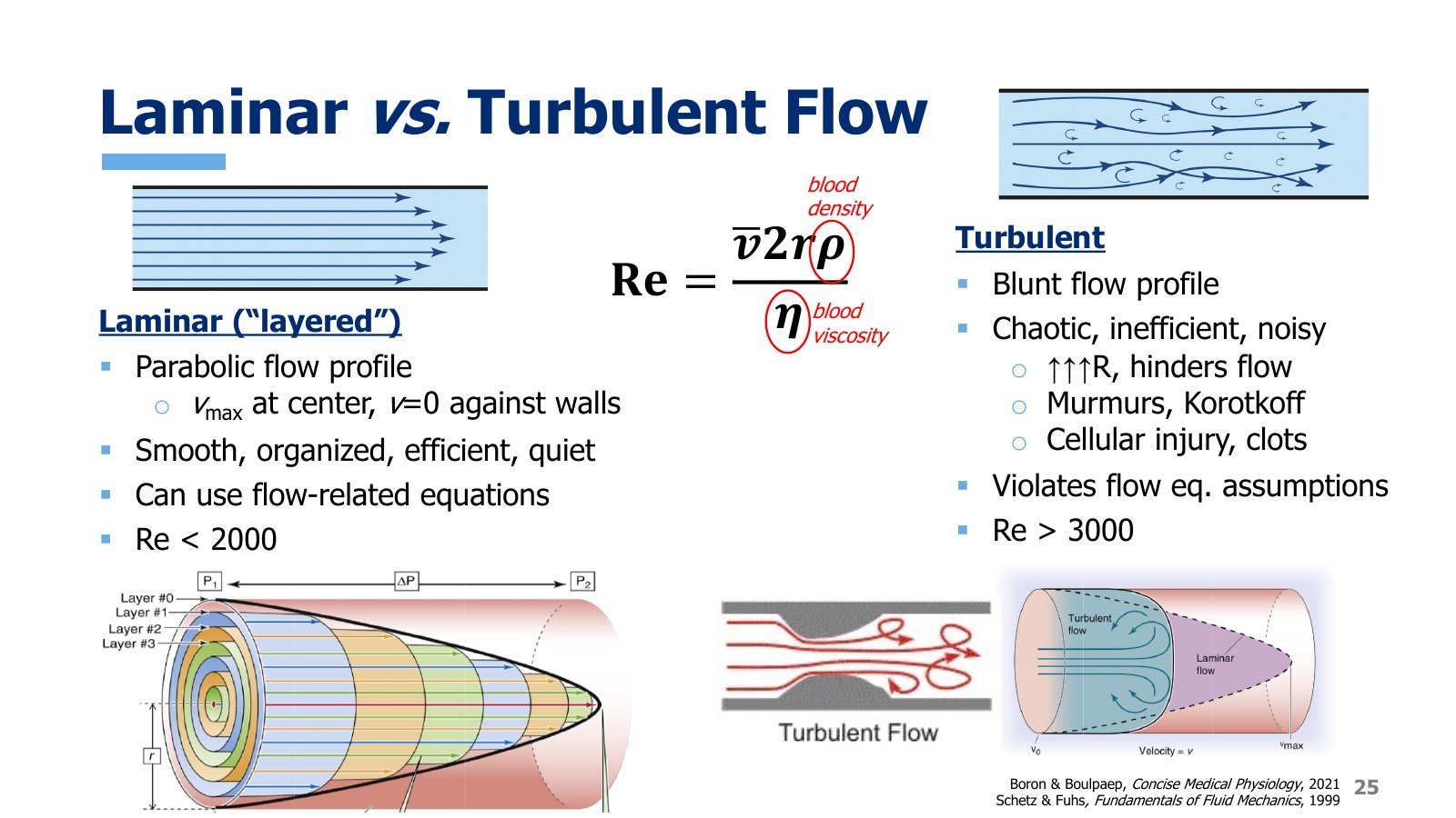
Slide 25. Left, laminar flow with its concentric layers and parabolic profile. Center, the Reynolds number. Right, turbulent flow with eddies and a blunt profile, including turbulence just past a narrowing.
Every equation and model of flow so far has relied on an important assumption: that flow is laminar. A lamina is a thin layer of something, so laminar describes the concentric layers of flow inside a blood vessel.
In the longitudinal section at top, the arrows look a little like lanes in a swimming pool, with the fastest swimmer in the middle and the swimmers getting slower out toward the edges. That is the nature of laminar flow. Flow travels in distinct, separated layers with minimal interaction with each other. The fastest flow is in the middle of the vessel, and velocity gets slower moving outward until the layer right next to the vessel wall has a velocity of zero.
The more three-dimensional figure below shows the layers arranged concentrically, each nested within the next outside layer. Again the fastest flow is in the center, and the layers slow toward the wall, giving a cone-like, parabolic flow profile.
In laminar flow, the layers all stay in their own lane and move forward together in an organized, coordinated, smooth, efficient manner. This flow is quiet and unobtrusive. Importantly, it is the type of flow that lets us use the flow-related equations in this module.
The Reynolds number
We can predict whether flow will be laminar under a given set of circumstances by calculating the Reynolds number, Re. For a vessel it equals mean blood velocity times vessel diameter (two times radius) times blood density, all divided by blood viscosity.
The Reynolds number has no units. If it comes out less than 2,000, flow is typically laminar. The equation tells us flow is more likely to stay organized and smooth when blood velocity is slower, when the vessel is smaller, and when blood viscosity is higher. Density may change in other applications of this equation in other contexts, but blood density doesn’t really change, so we mostly treat it as a constant here.
Turbulent flow
Turbulent flow has very different characteristics. The distinct layers break down, crossing into each other’s lanes and creating regions of swirling flow called eddies. Turbulent flow tends to have a blunter, flatter flow profile, with all layers at fairly similar velocities. That is because the layers interacting with each other homogenizes their velocities. As we lose the distinction between layers, we lose the differences in their velocities too.
Turbulent flow is chaotic, disorganized, inefficient, and noisy.
Inefficient. As the layers mix, kinetic energy is lost, or dissipated, hampering the forward flow of blood. Resistance increases dramatically, because it is just harder to move flow forward through the vessel.
Noisy. Not just metaphorically. Turbulent flow in the vessels can literally be heard by the human ear with a stethoscope. Heart valve disorders like stenosis or regurgitation create regions of turbulent flow around the diseased valve as blood passes through, and clinicians can preliminarily diagnose valvulopathy because they can hear the turbulence. These moments of turbulent flow in the cardiac cycle are murmurs. We also capitalize on the sound of arterial turbulence every time we take a blood pressure with a cuff. The sounds clinicians listen for are the Korotkoff sounds.
Damaging. Turbulence is a violent flow dynamic. For the cells most directly exposed to it, endothelial cells and red blood cells, it can lead to cellular damage and dysfunction, as well as clotting at the wrong times for the wrong reasons.
We need to predict whether flow is turbulent because none of our flow equations apply once it is. Blood flow through vessels typically becomes turbulent once the Reynolds number exceeds 3,000.
An abrupt change in vessel geometry can also create regions of turbulent flow: where vessels branch or bifurcate, or where blood meets an atherosclerotic plaque in the vessel wall that sticks out into the lumen a bit. The plaque developed there in the first place because there was already some endothelial damage in the wall, and the turbulent flow the plaque induces further damages the endothelium. It is a pathological downward spiral.
Laminar against turbulent flow
Feature | Laminar | Turbulent |
|---|---|---|
Layers | Distinct, stay in their own lane | Break down, cross lanes, form eddies |
Flow profile | Parabolic. Fastest at center, zero at the wall | Blunt and flat. Similar velocities across layers |
Character | Smooth, organized, efficient, quiet | Chaotic, disorganized, inefficient, noisy |
Resistance | Predicted by the flow equations | Increases dramatically |
Flow equations | Apply | Do not apply |
Reynolds number | < 2,000 |
|
Blood viscosity
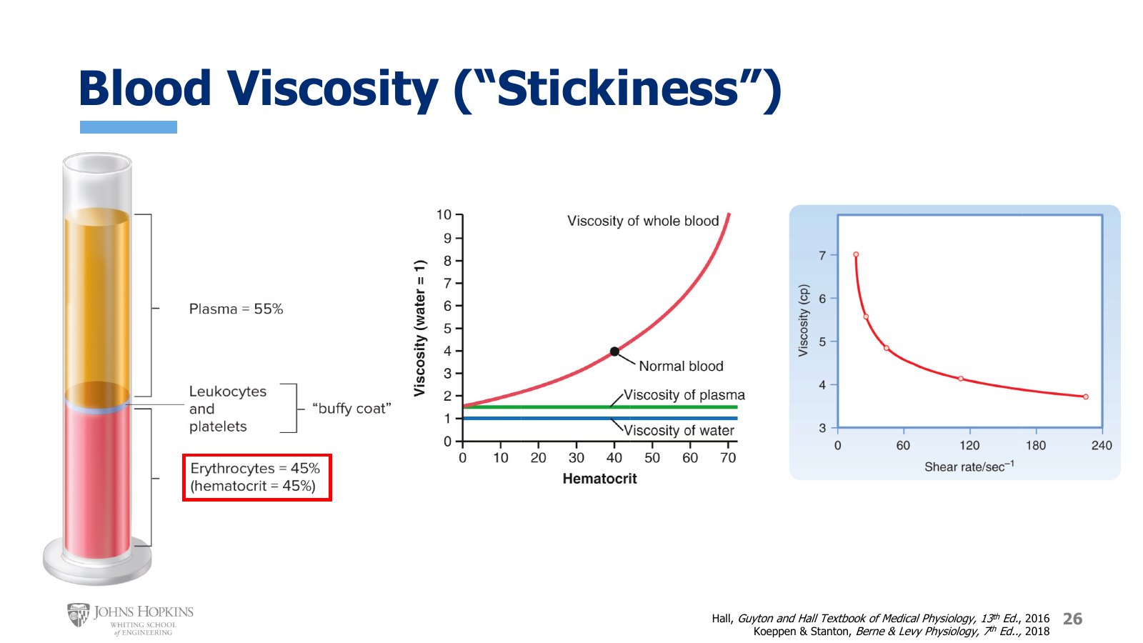
Slide 26. Left, centrifuged blood: plasma 55% on top, erythrocytes 45% below, and a thin buffy coat of leukocytes and platelets between. Center, whole blood viscosity rising with hematocrit against flat plasma and water. Right, viscosity falling as shear rate rises.
Blood viscosity is one of the factors that determines whether flow is laminar or turbulent. Viscosity is sometimes described as the thickness of a liquid, like honey or syrup, but it is more accurately the stickiness of the fluid: its cohesive tendency to stick to itself. Some of blood’s viscosity comes from molecular interactions in the plasma, like those between dissolved protein molecules. Most comes from the cellular portion of the blood, the red blood cells, which like to stick to each other.
Spin a tube of blood in a centrifuge and the heaviest elements, the cells, fall to the bottom of the tube while the lighter plasma comes to the top. Separating the liquid from the solid phase this way, plasma occupies roughly 55% of whole blood volume, and red blood cells, or erythrocytes, about 45%. The percent of blood volume occupied by red blood cells is a common clinical blood variable, hematocrit. A hematocrit of 45 means 45% of blood volume is red blood cells.
Hematocrit. Since the sticky interactions between red blood cells are responsible for most of blood’s viscosity, higher hematocrit leads to higher viscosity. Water’s viscosity is constant at 1 centipoise, and plasma’s is constant at around 1.3 centipoise, but the viscosity of whole blood, plasma and cells together, is variable and increases as a function of hematocrit.
Shear rate. Hematocrit isn’t the only factor. The shear rate, the difference in velocity between adjacent layers of flow, also influences viscosity.
Low shear rate. Very little difference in velocity between adjacent layers, so red blood cells in adjacent layers travel at roughly the same speed. They have more opportunity to interact, increasing the internal stickiness of the blood as a whole: higher viscosity.
High shear rate. A big enough difference in velocity between adjacent layers that cellular interactions are disrupted, decreasing the internal stickiness of the blood: lower viscosity.